Supervised Learning: Support Vector Machines

This is the 7th in a series of class notes as I go through the Georgia Tech/Udacity Machine Learning course. The class textbook is Machine Learning by Tom Mitchell.

Intuition for why

Drawing lines to separate between groups is actually a fairly weak condition. Now that we know how to boost our algorithms to arbitrary complexity, the next frontier to solve is choosing the “best” lines to draw. There are still a wide range of valid lines (aka weak learners) that completely separate groups, but subjectively some lines are better than others.

Given group A and group B, you’d prefer a line that is equidistant between A and B, rather than just barely on the border of either. The theory is that A and B are just samples of a larger population, so if you draw the lines too close to either, they will likely fail to generalize.

The other way to phrase this is that it is the hypothesis line that is supported by the data but commits the least to it.

Finding this optimal delineation is the intuition for SVMs.

Finding the margin

We find the widest possible band of possible space between groups, find a line that is perpendicular to each side of the band at each point, and choose the midpoint of the perpendicular line. We call this line the margin.

Formally, a classifier f can be boiled down to:

wX + b = C

where 

- b is a constant
- w is a simple, linear vector
- X is one or more dimensions of input variables
- C is the classifier output, either -1 or +1

So we can set up

wX1 + b = 1
wX2 + b = -1

for any two sets of X variables. The equation for the margin, or the perpendicular distance between them, (w/mod(w))X1-X2 gives us 2/mod(w), which is also the distance between the two planes. We want to maximize 2/mod(w) while classifying everything correctly, which is hard to solve, so we transform the problem to minimizing 1/2 * mod(w) ^ 2, which is a quadratic programming problem that we do know how to solve, with the same answer.

The solution looks like this:

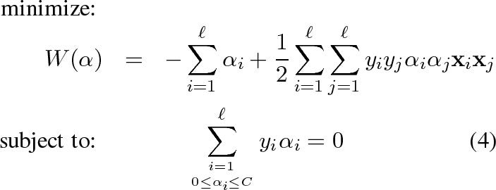
and you can check the associated post to further understand the alpha parameters.

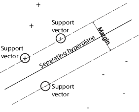
It turns out that the quadratic programming solution only relies on a few data points, the ones at the edge of the groups. In other words, most of the alpha parameters turn out to be near 0, except for those xi, xj combinations that are closes to the edges of the groups. This is intuitive - the points inside the groups simply don’t provide as much information as to where the boundary of the group is. We call these outer data points support vectors - as you can see here, these are the black dots closest to the lines:

Here’s another picture just to be sure:

This sounds a lot like K Nearest Neighbors! Except here you are finding separators for entire groups of datapoints.

The Kernel Trick

Inside the quadratic programming solution there is a projection between the two points on either side of the margin that involves a similarity score. In the simplest case it can be a simple dot product (0 if perpendicular, 1 if they point the same way, -1 if they point exactly opposite), but you can generalize it to almost any similarity function you can think of. This can be useful for adding dimensions to transform your existing data into linearly separable spaces.

So even though we can only draw straight lines with our SVM methods, and might be unable to draw lines for a given set of data, we can transform our datapoints so that lines -can- be drawn in the higher dimension:

Here, we were unable to draw a line in 2 dimensions to carve out the circle, but once we added an extra dimension it became an easy task. You can do this for almost anything:

What is cool is that the transformation doesn’t have to be explicit - if we choose the new dimension such that the total new datapoints’ dot product has a nice closed form (hard to get wrong), we can use that as our kernel instead of the linear dot product and we will be solving that optimization instead. There are any number of kernels to use:

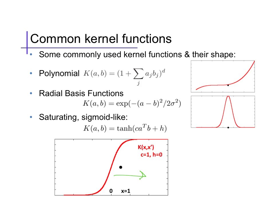
all with different characteristics. So your SVMs can even do this:

or this:

What ultimately matters is that your choice of kernel reflects your domain knowledge, your judgment of what datapoints (and projections of those datapoints) are valid members of the group based on features you identify, based on their similarity.

Side note: All SVM Kernels must satisfy the Mercer condition (a great answer as to why - basically, ensure that the matrix is PSD which means there is a global optimum to converge to)

SVMs and Boosting

In our Boosting chapter we talked about how Boosting tends not to overfit. We can introduce the idea of a difference between the concepts of error and confidence in our training results. In early stages of training, confidence goes up as error goes down. This is analogous to SVMs searching for and widening their margins, the wider the better.

However, what if we get to a point where no errors are left? (Because we have boosted our hypothesis so much we get perfect separation) Error is at 0, and has nowhere further to go. As we keep adding more and more weak learners, however, the confidence in our result continues to go up as the separation becomes clearer and clearer (we continue redraw the space in which we separate the two sides). The boostign algorithm is effectively continuing to widen the margin, which tends to minimize overfitting as we inferred above.

Boosting does overfit in some cases, for example when its learner is based on a very complex multilayered artificial neural network. In practice, this isn’t much of a concern.

Next in our series

Further notes on this topic:

• ICML tutorial on SVMs: https://www.cs.rochester.edu/~stefanko/Teaching/09CS446/SVM-ICML01-tutorial.pdf
• Burges’ SVMs for pattern recognition: http://research.microsoft.com/pubs/67119/svmtutorial.pdf
• Scholkopf’s SVMS and kernel methods: https://github.com/pushkar/4641/raw/master/downloads/svm-scholkopf.ps
• MIT’s SVM lecture: https://www.youtube.com/watch?v=_PwhiWxHK8o (recommended)
• An Idiot’s Guide to SVMs: http://web.mit.edu/6.034/wwwbob/svm-notes-long-08.pdf

Hopefully that was a good introduction to SVMs. I am planning more primers and would love your feedback and questions on:

• Overview
• Supervised Learning
  • Decision Trees
  • Regression
  • Neural Networks
  • Instance Based Learning (K Nearest Neighbors)
  • Ensemble Learning (AdaBoost)
  • Kernel Methods & SVMs
  • Computational Learning Theory
  • VC Dimensions
  • Bayesian Learning
  • Bayesian Inference
• Unsupervised Learning
  • Randomized Optimization
  • Information Theory
  • Clustering - week of Feb 25
  • Feature Selection - week of Mar 4
  • Feature Transformation - week of Mar 11
• Reinforcement Learning
  • Markov Decision Processes - week of Mar 25
  • “True” RL - week of Apr 1
  • Game Theory - week of Apr 15